Running Timefold Solver

1. The `Solver` interface

A Solver solves your planning problem.

Java

public interface Solver<Solution_> {

    Solution_ solve(Solution_ problem);

    ...
}

A Solver can only solve one planning problem instance at a time. It is built with a SolverFactory, there is no need to implement it yourself.

A Solver should only be accessed from a single thread, except for the methods that are specifically documented in javadoc as being thread-safe. The solve() method hogs the current thread. This can cause HTTP timeouts for REST services and it requires extra code to solve multiple datasets in parallel. To avoid such issues, use a SolverManager instead.

2. Solving a problem

Solving a problem is quite easy once you have:

A Solver built from a solver configuration
A @PlanningSolution that represents the planning problem instance

Just provide the planning problem as argument to the solve() method and it will return the best solution found:

Java

    Timetable problem = ...;
    Timetable bestSolution = solver.solve(problem);

In school timetabling, the solve() method will return a Timetable instance with every Lesson assigned to a Teacher and a Timeslot.

The solve(Solution) method can take a long time (depending on the problem size and the solver configuration). The Solver intelligently wades through the search space of possible solutions and remembers the best solution it encounters during solving. Depending on a number of factors (including problem size, how much time the Solver has, the solver configuration, …), that best solution might or might not be an optimal solution.

The solution instance given to the method solve(solution) is changed by the Solver, but do not mistake it for the best solution.

The solution instance returned by the methods solve(solution) or getBestSolution() is most likely a planning clone of the instance given to the method solve(solution), which implies it is a different instance.

The solution instance given to the solve(Solution) method may be partially or fully initialized, which is often the case in repeated planning.

2.1. Multi-threaded solving

There are several ways of running the solver in parallel:

Multi-threaded incremental solving: Solve 1 dataset with multiple threads without sacrificing incremental score calculation.
Partitioned search: Split 1 dataset in multiple parts and solve them independently.
Multi bet solving: solve 1 dataset with multiple, isolated solvers and take the best result.
- Not recommended: This is a marginal gain for a high cost of hardware resources.
- Use the Benchmarker during development to determine the algorithm that is the most appropriate on average.
Multitenancy: solve different datasets in parallel.
- The SolverManager can help with this.

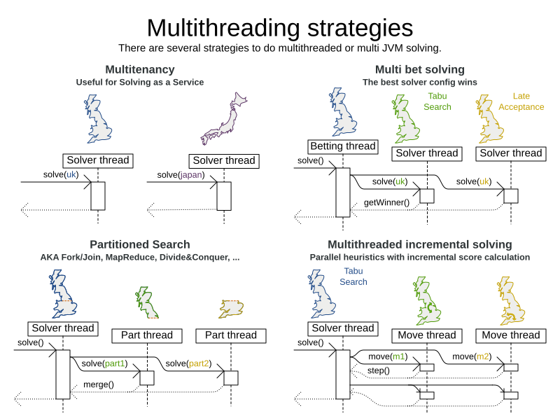
2.1.1. Multi-threaded incremental solving

This feature is exclusive to Timefold Solver Enterprise Edition.

With this feature, the solver can run significantly faster, getting you the right solution earlier. It has been designed to speed up the solver in cases where move evaluation is the bottleneck. This typically happens when the constraints are computationally expensive, or when the dataset is large.

The sweet spot for this feature is when the move evaluation speed is up to 10 thousand per second. In this case, we have observed the algorithm to scale linearly with the number of move threads. Every additional move thread will bring a speedup, albeit with diminishing returns.
For move evaluation speeds on the order of 100 thousand per second, the algorithm no longer scales linearly, but using 4 to 8 move threads may still be beneficial.
For even higher move evaluation speeds, the feature does not bring any benefit. At these speeds, move evaluation is no longer the bottleneck. If the solver continues to underperform, perhaps you’re suffering from score traps or you may benefit from custom moves to help the solver escape local optima.

These guidelines are strongly dependent on move selector configuration, size of the dataset and performance of individual constraints. We recommend you benchmark your use case to determine the optimal number of move threads for your problem.

Enabling multi-threaded incremental solving

Enable multi-threaded incremental solving by adding a @PlanningId annotation on every planning entity class and planning value class. Then configure a moveThreadCount:

Quarkus
Spring
Java
XML

Add the following to your application.properties:

quarkus.timefold.solver.move-thread-count=AUTO

Add the following to your application.properties:

timefold.solver.move-thread-count=AUTO

Use the SolverConfig class:

SolverConfig solverConfig = new SolverConfig()
    ...
    .withMoveThreadCount("AUTO");

Add the following to your solverConfig.xml:

<solver xmlns="https://timefold.ai/xsd/solver" xmlns:xsi="http://www.w3.org/2001/XMLSchema-instance"
xsi:schemaLocation="https://timefold.ai/xsd/solver https://timefold.ai/xsd/solver/solver.xsd">

    ...
    <moveThreadCount>AUTO</moveThreadCount>
    ...

</solver>

Setting moveThreadCount to AUTO allows Timefold Solver to decide how many move threads to run in parallel. This formula is based on experience and does not hog all CPU cores on a multi-core machine.

A moveThreadCount of 4 saturates almost 5 CPU cores. The 4 move threads fill up 4 CPU cores completely and the solver thread uses most of another CPU core.

The following moveThreadCounts are supported:

NONE (default): Don’t run any move threads. Use the single threaded code.
AUTO: Let Timefold Solver decide how many move threads to run in parallel. On machines or containers with little or no CPUs, this falls back to the single threaded code.
Static number: The number of move threads to run in parallel.

It is counter-effective to set a moveThreadCount that is higher than the number of available CPU cores, as that will slow down the move evaluation speed.

In cloud environments where resource use is billed by the hour, consider the trade-off between cost of the extra CPU cores needed and the time saved. Compute nodes with higher CPU core counts are typically more expensive to run and therefore you may end up paying more for the same result, even though the actual compute time needed will be less.

Multi-threaded solving is still reproducible, as long as the resolved moveThreadCount is stable. A run of the same solver configuration on 2 machines with a different number of CPUs, is still reproducible, unless the moveThreadCount is set to AUTO or a function of availableProcessorCount.

Advanced configuration

There are additional parameters you can supply to your solverConfig.xml:

<solver xmlns="https://timefold.ai/xsd/solver" xmlns:xsi="http://www.w3.org/2001/XMLSchema-instance"
    xsi:schemaLocation="https://timefold.ai/xsd/solver https://timefold.ai/xsd/solver/solver.xsd">
  <moveThreadCount>4</moveThreadCount>
  <threadFactoryClass>...MyAppServerThreadFactory</threadFactoryClass>
  ...
</solver>

To run in an environment that doesn’t like arbitrary thread creation, use threadFactoryClass to plug in a custom thread factory.

2.1.2. Partitioned search

This feature is exclusive to Timefold Solver Enterprise Edition.

Algorithm description

It is often more efficient to partition large data sets (usually above 5000 planning entities) into smaller pieces and solve them separately. Partition Search is multi-threaded, so it provides a performance boost on multi-core machines due to higher CPU utilization. Additionally, even when only using one CPU, it finds an initial solution faster, because the search space sum of a partitioned Construction Heuristic is far less than its non-partitioned variant.

However, partitioning does lead to suboptimal results, even if the pieces are solved optimally, as shown below:

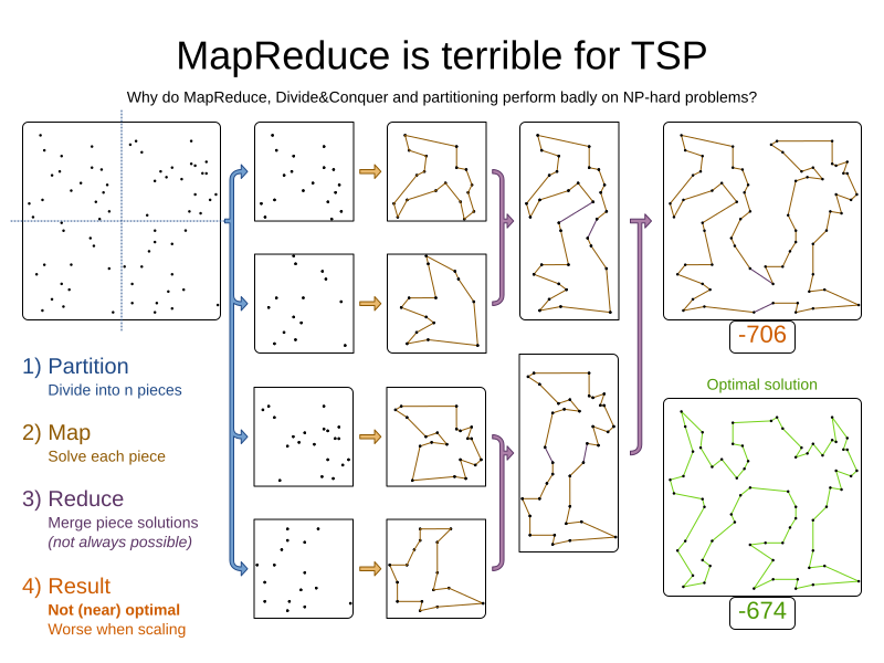
It effectively trades a short term gain in solution quality for long term loss. One way to compensate for this loss, is to run a non-partitioned Local Search after the Partitioned Search phase.

Not all use cases can be partitioned. Partitioning only works for use cases where the planning entities and value ranges can be split into n partitions, without any of the constraints crossing boundaries between partitions.

Configuration

Simplest configuration:

  <partitionedSearch>
    <solutionPartitionerClass>...MyPartitioner</solutionPartitionerClass>
  </partitionedSearch>

Also add a @PlanningId annotation on every planning entity class and planning value class. There are several ways to partition a solution.

Advanced configuration:

  <partitionedSearch>
    ...
    <solutionPartitionerClass>...MyPartitioner</solutionPartitionerClass>
    <runnablePartThreadLimit>4</runnablePartThreadLimit>

    <constructionHeuristic>...</constructionHeuristic>
    <localSearch>...</localSearch>
  </partitionedSearch>

The runnablePartThreadLimit allows limiting CPU usage to avoid hanging your machine, see below.

To run in an environment that doesn’t like arbitrary thread creation, plug in a custom thread factory.

A logging level of debug or trace causes congestion in multi-threaded Partitioned Search and slows down the move evaluation speed.

Just like a <solver> element, the <partitionedSearch> element can contain one or more phases. Each of those phases will be run on each partition.

A common configuration is to first run a Partitioned Search phase (which includes a Construction Heuristic and a Local Search) followed by a non-partitioned Local Search phase:

  <partitionedSearch>
    <solutionPartitionerClass>...MyPartitioner</solutionPartitionerClass>

    <constructionHeuristic/>
    <localSearch>
      <termination>
        <diminishedReturns />
      </termination>
    </localSearch>
  </partitionedSearch>
  <localSearch/>

Partitioning a solution

Custom `SolutionPartitioner`

To use a custom SolutionPartitioner, configure one on the Partitioned Search phase:

  <partitionedSearch>
    <solutionPartitionerClass>...MyPartitioner</solutionPartitionerClass>
  </partitionedSearch>

Implement the SolutionPartitioner interface:

public interface SolutionPartitioner<Solution_> {

    List<Solution_> splitWorkingSolution(Solution_ workingSolution, Integer runnablePartThreadLimit);

}

The size() of the returned List is the partCount (the number of partitions). This can be decided dynamically, for example, based on the size of the non-partitioned solution. The partCount is unrelated to the runnablePartThreadLimit.

To configure values of a SolutionPartitioner dynamically in the solver configuration (so the Benchmarker can tweak those parameters), add the solutionPartitionerCustomProperties element and use custom properties:

  <partitionedSearch>
    <solutionPartitionerClass>...MyPartitioner</solutionPartitionerClass>
    <solutionPartitionerCustomProperties>
      <property name="myPartCount" value="8"/>
      <property name="myMinimumProcessListSize" value="100"/>
    </solutionPartitionerCustomProperties>
  </partitionedSearch>

Runnable part thread limit

When running a multi-threaded solver, such as Partitioned Search, CPU power can quickly become a scarce resource, which can cause other processes or threads to hang or freeze. However, Timefold Solver has a system to prevent CPU starving of other processes (such as an SSH connection in production or your IDE in development) or other threads (such as the servlet threads that handle REST requests).

As explained in sizing hardware and software, each solver (including each child solver) does no IO during solve() and therefore saturates one CPU core completely. In Partitioned Search, every partition always has its own thread, called a part thread. It is impossible for two partitions to share a thread, because of asynchronous termination: the second thread would never run. Every part thread will try to consume one CPU core entirely, so if there are more partitions than CPU cores, this will probably hang the system. Thread.setPriority() is often too weak to solve this hogging problem, so another approach is used.

The runnablePartThreadLimit parameter specifies how many part threads are runnable at the same time. The other part threads will temporarily block and therefore will not consume any CPU power. This parameter basically specifies how many CPU cores are donated to Timefold Solver. All part threads share the CPU cores in a round-robin manner to consume (more or less) the same number of CPU cycles:

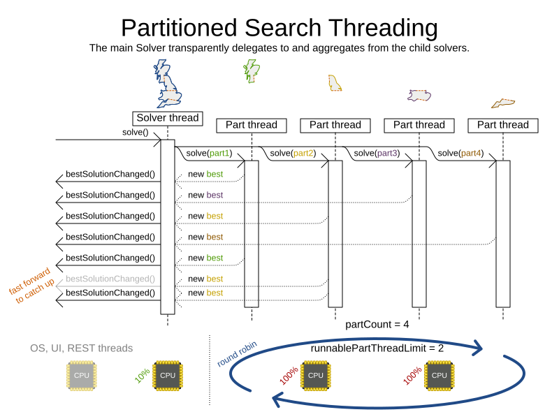
The following runnablePartThreadLimit options are supported:

UNLIMITED: Allow Timefold Solver to occupy all CPU cores, do not avoid hogging. Useful if a no hogging CPU policy is configured on the OS level.
AUTO (default): Let Timefold Solver decide how many CPU cores to occupy. This formula is based on experience. It does not hog all CPU cores on a multi-core machine.
Static number: The number of CPU cores to consume. For example:
```
<runnablePartThreadLimit>2</runnablePartThreadLimit>
```

If the runnablePartThreadLimit is equal to or higher than the number of available processors, the host is likely to hang or freeze, unless there is an OS specific policy in place to avoid Timefold Solver from hogging all the CPU processors.

2.1.3. Custom thread factory (WildFly, GAE, …)

The threadFactoryClass allows to plug in a custom ThreadFactory for environments where arbitrary thread creation should be avoided, such as most application servers (including WildFly) or Google App Engine.

Configure the ThreadFactory on the solver to create the move threads and the Partition Search threads with it:

<solver xmlns="https://timefold.ai/xsd/solver" xmlns:xsi="http://www.w3.org/2001/XMLSchema-instance"
    xsi:schemaLocation="https://timefold.ai/xsd/solver https://timefold.ai/xsd/solver/solver.xsd">
  <threadFactoryClass>...MyAppServerThreadFactory</threadFactoryClass>
  ...
</solver>

3. Environment mode: are there bugs in my code?

The environment mode allows you to detect common bugs in your implementation. It does not affect the logging level.

You can set the environment mode in the solver configuration XML file:

<solver xmlns="https://timefold.ai/xsd/solver" xmlns:xsi="http://www.w3.org/2001/XMLSchema-instance"
    xsi:schemaLocation="https://timefold.ai/xsd/solver https://timefold.ai/xsd/solver/solver.xsd">
  <environmentMode>STEP_ASSERT</environmentMode>
  ...
</solver>

A solver has a single Random instance. Some solver configurations use the Random instance a lot more than others. For example, Simulated Annealing depends highly on random numbers, while Tabu Search only depends on it to deal with score ties. The environment mode influences the seed of that Random instance.

3.1. Reproducibility

For the environment mode to be reproducible, any two runs of the same dataset with the same solver configuration must have the same result at every step. Choosing a reproducible environment mode enables you to reproduce bugs consistently. It also allows you to benchmark certain refactorings (such as a score constraint performance optimization) fairly across runs.

Regardless of whether the chosen environment mode itself is reproducible, your application might still not be fully reproducible because of:

Use of HashSet (or another Collection which has an undefined iteration order between JVM runs) for collections of planning entities or planning values (but not normal problem facts), especially in the solution implementation. Replace it with a SequencedSet or SequencedCollection implementation respectively, such as LinkedHashSet or ArrayList.
- This also applies to HashMap, which can be replaced by a SequencedMap implementation such as LinkedHashMap.
Combining a time gradient-dependent algorithm (most notably Simulated Annealing) together with time spent termination. A large enough difference in allocated CPU time will influence the time gradient values. Replace Simulated Annealing with Late Acceptance, or replace time spent termination with step count termination.

3.2. Available environment modes

The following environment modes are available, in the order from least strict to most strict:

NON_REPRODUCIBLE
NO_ASSERT
PHASE_ASSERT (default)
STEP_ASSERT
NON_INTRUSIVE_FULL_ASSERT
FULL_ASSERT
TRACKED_FULL_ASSERT

As the environment mode becomes stricter, the solver becomes slower, but gains more error-detection capabilities. STEP_ASSERT is already slow enough to prevent its use in production.

All modes other than NON_REPRODUCIBLE are reproducible.

3.2.1. `TRACKED_FULL_ASSERT`

The TRACKED_FULL_ASSERT mode turns on all the FULL_ASSERT assertions and additionally tracks changes to the working solution. This allows the solver to report exactly what variables were corrupted.

In particular, the solver will recalculate all shadow variables from scratch on the solution after the undo and then report:

Genuine and shadow variables that are different between "before" and "undo". After an undo move is evaluated, it is expected to exactly match the original working solution.
Variables that are different between "from scratch" and "before". This is to detect if the solution was corrupted before the move was evaluated due to shadow variable corruption.
Variables that are different between "from scratch" and "undo". This is to detect if recalculating the shadow variables from scratch is different from the incremental shadow variable calculation.
Missing variable events for the actual move. Any variable that changed between the "before move" solution and the "after move" solution without the solver being notified of the change.
Missing events for undo move. Any variable that changed between the "after move" solution and "after undo move" solution without the solver being notified of the change.

This mode is reproducible (see the reproducible mode). It is also intrusive because it calls the method calculateScore() more frequently than a non-assert mode.

The TRACKED_FULL_ASSERT mode is by far the slowest mode, because it clones solutions before and after each move.

3.2.2. `FULL_ASSERT`

The FULL_ASSERT mode turns on all assertions and will fail-fast on a bug in a Move implementation, a constraint, the engine itself, … It is also intrusive because it calls the method calculateScore() more frequently than a NO_ASSERT mode, making the FULL_ASSERT mode very slow.

This mode is reproducible.

This mode is neither better nor worse than NON_INTRUSIVE_FULL_ASSERT - each can catch different types of errors, on account of performing score calculations at different times.

3.2.3. `NON_INTRUSIVE_FULL_ASSERT`

The NON_INTRUSIVE_FULL_ASSERT mode turns on most assertions and will fail-fast on a bug in a Move implementation, a constraint, the engine itself, … It is not intrusive, as it does not call the method calculateScore() more frequently than a NO_ASSERT mode.

This mode is reproducible. This mode is also very slow, on account of all the additional checks performed.

This mode is neither better nor worse than FULL_ASSERT - each can catch different types of errors, on account of performing score calculations at different times.

3.2.4. `STEP_ASSERT`

The STEP_ASSERT mode turns on most assertions (such as assert that an undoMove’s score is the same as before the Move) to fail-fast on a bug in a Move implementation, a constraint, the engine itself, … This makes it slow.

This mode is reproducible. It is also intrusive because it calls the method calculateScore() more frequently than a non-assert mode.

We recommend that you write a test case that does a short run of your planning problem with the STEP_ASSERT mode on.

3.2.5. `PHASE_ASSERT` (default)

The PHASE_ASSERT is the default mode because it is recommended during development. This mode is reproducible and it gives you the benefit of quickly checking for score corruptions. If you can guarantee that your code is and will remain bug-free, you can switch to the NO_ASSERT mode for a marginal performance gain.

In practice, this mode disables certain concurrency optimizations, such as work stealing.

3.2.6. `NO_ASSERT`

The NO_ASSERT environment mode behaves in all aspects like the default PHASE_ASSERT mode, except that it does not give you any protection against score corruption bugs. As such, it can be negligibly faster.

3.2.7. `NON_REPRODUCIBLE`

This mode can be slightly faster than any of the other modes, but it is not reproducible. Avoid using it during development as it makes debugging and bug fixing painful. If your production environment doesn’t care about reproducibility, use this mode in production.

Unlike all the other modes, this mode doesn’t use any fixed random seed unless one is provided.

3.3. Best practices

There are several best practices to follow throughout the lifecycle of your application:

In production

Use the PHASE_ASSERT mode if you need reproducibility, otherwise use NON_REPRODUCIBLE.

In development

Use the PHASE_ASSERT mode to catch bugs early.
Write a test case that does a short run of your planning problem in STEP_ASSERT mode.
Have nightly builds that run for several minutes in FULL_ASSERT and NON_INTRUSIVE_FULL_ASSERT modes.

4. Logging level: what is the `Solver` doing?

The best way to illuminate the black box that is a Solver, is to play with the logging level:

error: Log errors, except those that are thrown to the calling code as a RuntimeException.

If an error happens, Timefold Solver normally fails fast: it throws a subclass of RuntimeException with a detailed message to the calling code. It does not log it as an error itself to avoid duplicate log messages. Except if the calling code explicitly catches and eats that RuntimeException, a Thread's default ExceptionHandler will log it as an error anyway. Meanwhile, the code is disrupted from doing further harm or obfuscating the error.

warn: Log suspicious circumstances.
info: Log every phase and the solver itself. See scope overview.
debug: Log every step of every phase. See scope overview.
trace: Log every move of every step of every phase. See scope overview.

Turning on trace logging, will slow down performance considerably: it is often four times slower. However, it is invaluable during development to discover a bottleneck.

Even debug logging can slow down performance considerably for fast stepping algorithms (such as Late Acceptance and Simulated Annealing), but not for slow stepping algorithms (such as Tabu Search).

Both trace logging and debug logging cause congestion in multi-threaded solving with most appenders, see below.

In Eclipse, debug logging to the console tends to cause congestion with move evaluation speeds above 10 000 per second. Nor IntelliJ, nor the Maven command line suffer from this problem.

For example, set it to debug logging, to see when the phases end and how fast steps are taken:

INFO  Solving started: time spent (31), best score (0hard/0soft), environment mode (PHASE_ASSERT), move thread count (NONE), random (JDK with seed 0).
INFO  Problem scale: entity count (4), variable count (8), approximate value count (4), approximate problem scale (256).
DEBUG     CH step (0), time spent (47), score (0hard/0soft), selected move count (4), picked move ([Math(0) {null -> Room A}, Math(0) {null -> MONDAY 08:30}]).
DEBUG     CH step (1), time spent (50), score (0hard/0soft), selected move count (4), picked move ([Physics(1) {null -> Room A}, Physics(1) {null -> MONDAY 09:30}]).
DEBUG     CH step (2), time spent (51), score (-1hard/-1soft), selected move count (4), picked move ([Chemistry(2) {null -> Room B}, Chemistry(2) {null -> MONDAY 08:30}]).
DEBUG     CH step (3), time spent (52), score (-2hard/-1soft), selected move count (4), picked move ([Biology(3) {null -> Room A}, Biology(3) {null -> MONDAY 08:30}]).
INFO  Construction Heuristic phase (0) ended: time spent (53), best score (-2hard/-1soft), move evaluation speed (1066/sec), step total (4).
DEBUG     LS step (0), time spent (56), score (-2hard/0soft), new best score (-2hard/0soft), accepted/selected move count (1/1), picked move (Chemistry(2) {Room B, MONDAY 08:30} <-> Physics(1) {Room A, MONDAY 09:30}).
DEBUG     LS step (1), time spent (60), score (-2hard/1soft), new best score (-2hard/1soft), accepted/selected move count (1/2), picked move (Math(0) {Room A, MONDAY 08:30} <-> Physics(1) {Room B, MONDAY 08:30}).
DEBUG     LS step (2), time spent (60), score (-2hard/0soft),     best score (-2hard/1soft), accepted/selected move count (1/1), picked move (Math(0) {Room B, MONDAY 08:30} <-> Physics(1) {Room A, MONDAY 08:30}).
...
INFO  Local Search phase (1) ended: time spent (100), best score (0hard/1soft), move evaluation speed (2021/sec), step total (59).
INFO  Solving ended: time spent (100), best score (0hard/1soft), move evaluation speed (1100/sec), phase total (2), environment mode (PHASE_ASSERT), move thread count (NONE).

All time spent values are in milliseconds.

Java

Everything is logged to SLF4J, which is a simple logging facade which delegates every log message to Logback, Apache Commons Logging, Log4j or java.util.logging. Add a dependency to the logging adaptor for your logging framework of choice.

If you are not using any logging framework yet, use Logback by adding this Maven dependency (there is no need to add an extra bridge dependency):

    <dependency>
      <groupId>ch.qos.logback</groupId>
      <artifactId>logback-classic</artifactId>
      <version>1.x</version>
    </dependency>

Configure the logging level on the ai.timefold.solver package in your logback.xml file:

<configuration>

  <logger name="ai.timefold.solver" level="debug"/>

  ...

</configuration>

If it isn’t picked up, temporarily add the system property -Dlogback.debug=true to figure out why.

When running multiple solvers or a multi-threaded solver, most appenders (including the console) cause congestion with debug and trace logging. Switch to an async appender to avoid this problem or turn off debug logging.

In a multitenant application, multiple Solver instances might be running at the same time. To separate their logging into distinct files, surround the solve() call with an MDC:

        MDC.put("tenant.name", tenantName);
        MySolution bestSolution = solver.solve(problem);
        MDC.remove("tenant.name");

Then configure your logger to use different files for each ${tenant.name}. In Logback, use a SiftingAppender in logback.xml:

  <appender name="fileAppender" class="ch.qos.logback.classic.sift.SiftingAppender">
    <discriminator>
      <key>tenant.name</key>
      <defaultValue>unknown</defaultValue>
    </discriminator>
    <sift>
      <appender name="fileAppender.${tenant.name}" class="...FileAppender">
        <file>local/log/timefold-solver-${tenant.name}.log</file>
        ...
      </appender>
    </sift>
  </appender>

5. Monitoring the solver

Timefold Solver exposes metrics through Micrometer which you can use to monitor the solver. Timefold automatically connects to configured registries when it is used in Quarkus or Spring Boot. If you use Timefold with plain Java, you must add the metrics registry to the global registry.

Prerequisites

You have a plain Java Timefold Solver project.
You have configured a Micrometer registry. For information about configuring Micrometer registries, see the Micrometer web site.

Procedure

Add configuration information for the Micrometer registry for your desired monitoring system to the global registry.

Add the following line below the configuration information, where <REGISTRY> is the name of the registry that you configured:

Metrics.addRegistry(<REGISTRY>);

The following example shows how to add the Prometheus registry:

PrometheusMeterRegistry prometheusRegistry = new PrometheusMeterRegistry(PrometheusConfig.DEFAULT);

try {
    HttpServer server = HttpServer.create(new InetSocketAddress(8080), 0);
    server.createContext("/prometheus", httpExchange -> {
        String response = prometheusRegistry.scrape(); (1)
        httpExchange.sendResponseHeaders(200, response.getBytes().length);
        try (OutputStream os = httpExchange.getResponseBody()) {
            os.write(response.getBytes());
        }
    });

    new Thread(server::start).start();
} catch (IOException e) {
    throw new RuntimeException(e);
}

Metrics.addRegistry(prometheusRegistry);

Open your monitoring system to view the metrics for your Timefold Solver project. The following metrics are exposed:

The names and format of the metrics vary depending on the registry.
- timefold.solver.errors.total: the total number of errors that occurred while solving since the start of the measuring.
- timefold.solver.solve.duration.active-count: the number of solvers currently solving.
- timefold.solver.solve.duration.seconds-max: run time of the longest-running currently active solver.
- timefold.solver.solve.duration.seconds-duration-sum: the sum of each active solver’s solve duration. For example, if there are two active solvers, one running for three minutes and the other for one minute, the total solve time is four minutes.

5.1. Additional metrics

For more detailed monitoring, Timefold Solver can be configured to monitor additional metrics at a performance cost.

<solver xmlns="https://timefold.ai/xsd/solver" xmlns:xsi="http://www.w3.org/2001/XMLSchema-instance"
    xsi:schemaLocation="https://timefold.ai/xsd/solver https://timefold.ai/xsd/solver/solver.xsd">
  <monitoring>
    <metric>BEST_SCORE</metric>
    <metric>SCORE_CALCULATION_COUNT</metric>
    ...
  </monitoring>
  ...
</solver>

The following metrics are available:

SOLVE_DURATION (default, Micrometer meter id: "timefold.solver.solve.duration"): Measurse the duration of solving for the longest active solver, the number of active solvers and the cumulative duration of all active solvers.
ERROR_COUNT (default, Micrometer meter id: "timefold.solver.errors"): Measures the number of errors that occur while solving.
SCORE_CALCULATION_COUNT (default, Micrometer meter id: "timefold.solver.score.calculation.count"): Measures the number of score calculations Timefold Solver performed.
MOVE_EVALUATION_COUNT (default, Micrometer meter id: "timefold.solver.move.evaluation.count"): Measures the number of move evaluations Timefold Solver performed.
PROBLEM_ENTITY_COUNT (default, Micrometer meter id: "timefold.solver.problem.entities"): Measures the number of entities in the problem submitted to Timefold Solver.
PROBLEM_VARIABLE_COUNT (default, Micrometer meter id: "timefold.solver.problem.variables"): Measures the number of genuine variables in the problem submitted to Timefold Solver.
PROBLEM_VALUE_COUNT (default, Micrometer meter id: "timefold.solver.problem.values"): Measures the approximate number of planning values in the problem submitted to Timefold Solver.
PROBLEM_SIZE_LOG (default, Micrometer meter id: "timefold.solver.problem.size.log"): Measures the approximate log 10 of the search space size for the problem submitted to Timefold Solver.
BEST_SCORE (Micrometer meter id: "timefold.solver.best.score.*"): Measures the score of the best solution Timefold Solver found so far. There are separate meters for each level of the score. For instance, for a HardSoftScore, there are timefold.solver.best.score.hard.score and timefold.solver.best.score.soft.score meters.
STEP_SCORE (Micrometer meter id: "timefold.solver.step.score.*"): Measures the score of each step Timefold Solver takes. There are separate meters for each level of the score. For instance, for a HardSoftScore, there are timefold.solver.step.score.hard.score and timefold.solver.step.score.soft.score meters.
BEST_SOLUTION_MUTATION (Micrometer meter id: "timefold.solver.best.solution.mutation"): Measures the number of changed planning variables between consecutive best solutions.
MOVE_COUNT_PER_STEP (Micrometer meter id: "timefold.solver.step.move.count"): Measures the number of moves evaluated in a step.
MOVE_COUNT_PER_TYPE (Micrometer meter id: "timefold.solver.move.type.count"): Measures the number of moves evaluated per move type.
MEMORY_USE (Micrometer meter id: "jvm.memory.used"): Measures the amount of memory used across the JVM. This does not measure the amount of memory used by a solver; two solvers on the same JVM will report the same value for this metric.
CONSTRAINT_MATCH_TOTAL_BEST_SCORE (Micrometer meter id: "timefold.solver.constraint.match.best.score.*"): Measures the score impact of each constraint on the best solution Timefold Solver found so far. There are separate meters for each level of the score, with tags for each constraint. For instance, for a HardSoftScore for a constraint "Minimize Cost", there are timefold.solver.constraint.match.best.score.hard.score and timefold.solver.constraint.match.best.score.soft.score meters with a tag "constraint.id=Minimize Cost".
CONSTRAINT_MATCH_TOTAL_STEP_SCORE (Micrometer meter id: "timefold.solver.constraint.match.step.score.*"): Measures the score impact of each constraint on the current step. There are separate meters for each level of the score, with tags for each constraint. For instance, for a HardSoftScore for a constraint "Minimize Cost", there are timefold.solver.constraint.match.step.score.hard.score and timefold.solver.constraint.match.step.score.soft.score meters with a tag "constraint.id=Minimize Cost".
PICKED_MOVE_TYPE_BEST_SCORE_DIFF (Micrometer meter id: "timefold.solver.move.type.best.score.diff.*"): Measures how much a particular move type improves the best solution. There are separate meters for each level of the score, with a tag for the move type. For instance, for a HardSoftScore and a ChangeMove for the room of a lesson, there are timefold.solver.move.type.best.score.diff.hard.score and timefold.solver.move.type.best.score.diff.soft.score meters with the tag move.type=ChangeMove(Lesson.room).
PICKED_MOVE_TYPE_STEP_SCORE_DIFF (Micrometer meter id: "timefold.solver.move.type.step.score.diff.*"): Measures how much a particular move type improves the best solution. There are separate meters for each level of the score, with a tag for the move type. For instance, for a HardSoftScore and a ChangeMove for the room of a lesson, there are timefold.solver.move.type.step.score.diff.hard.score and timefold.solver.move.type.step.score.diff.soft.score meters with the tag move.type=ChangeMove(Lesson.room).

6. Random number generator

Many heuristics and metaheuristics depend on a pseudorandom number generator for move selection, to resolve score ties, probability based move acceptance, … During solving, the same Random instance is reused to improve reproducibility, performance and uniform distribution of random values.

To change the random seed of that Random instance, specify a randomSeed:

<solver xmlns="https://timefold.ai/xsd/solver" xmlns:xsi="http://www.w3.org/2001/XMLSchema-instance"
    xsi:schemaLocation="https://timefold.ai/xsd/solver https://timefold.ai/xsd/solver/solver.xsd">
  <randomSeed>0</randomSeed>
  ...
</solver>

To change the pseudorandom number generator implementation, specify a randomType:

<solver xmlns="https://timefold.ai/xsd/solver" xmlns:xsi="http://www.w3.org/2001/XMLSchema-instance"
    xsi:schemaLocation="https://timefold.ai/xsd/solver https://timefold.ai/xsd/solver/solver.xsd">
  <randomType>MERSENNE_TWISTER</randomType>
  ...
</solver>

The following types are supported:

JDK (default): Standard implementation (java.util.Random).
MERSENNE_TWISTER: Implementation by Commons Math.
WELL512A, WELL1024A, WELL19937A, WELL19937C, WELL44497A and WELL44497B: Implementation by Commons Math.

For most use cases, the randomType has no significant impact on the average quality of the best solution on multiple datasets. If you want to confirm this on your use case, use the benchmarker.

7. `SolverManager`

A SolverManager is a facade for one or more Solver instances to simplify solving planning problems in REST and other enterprise services. Unlike the Solver.solve(…) method:

SolverManager.solve(…) returns immediately: it schedules a problem for asynchronous solving without blocking the calling thread. This avoids timeout issues of HTTP and other technologies.
SolverManager.solve(…) solves multiple planning problems of the same domain, in parallel.

Internally a SolverManager manages a thread pool of solver threads, which call Solver.solve(…), and a thread pool of consumer threads, which handle best solution changed events.

In Quarkus and Spring Boot, the SolverManager instance is automatically injected in your code. Otherwise, build a SolverManager instance with the create(…) method:

Java

SolverConfig solverConfig = SolverConfig.createFromXmlResource(".../solverConfig.xml");
SolverManager<VehicleRoutePlan, String> solverManager = SolverManager.create(solverConfig, new SolverManagerConfig());

Each problem submitted to the SolverManager.solve(…) methods needs a unique problem ID. Later calls to getSolverStatus(problemId) or terminateEarly(problemId) use that problem ID to distinguish between the planning problems. The problem ID must be an immutable class, such as Long, String or java.util.UUID.

The SolverManagerConfig class has a parallelSolverCount property, that controls how many solvers are run in parallel. For example, if set to 4, submitting five problems has four problems solving immediately, and the fifth one starts when another one ends. If those problems solve for 5 minutes each, the fifth problem takes 10 minutes to finish. By default, parallelSolverCount is set to AUTO, which resolves to half the CPU cores, regardless of the moveThreadCount of the solvers.

To retrieve the best solution, after solving terminates normally, use SolverJob.getFinalBestSolution():

Java

VehicleRoutePlan problem1 = ...;
String problemId = UUID.randomUUID().toString();
// Returns immediately
SolverJob<VehicleRoutePlan, String> solverJob = solverManager.solve(problemId, problem1);
...

try {
    // Returns only after solving terminates
    VehicleRoutePlan solution1 = solverJob.getFinalBestSolution();
} catch (InterruptedException | ExecutionException e) {
    throw ...;
}

However, there are better approaches, both for solving batch problems before an end-user needs the solution as well as for live solving while an end-user is actively waiting for the solution, as explained below.

The current SolverManager implementation runs on a single computer node, but future work aims to distribute solver loads across a cloud.

8. The `SolverManager` Builder

The SolverManager also enables the creation of a builder to customize and submit a planning problem for solving.

Java

public interface SolverManager<Solution_> {

    SolverJobBuilder<Solution_, ProblemId_> solveBuilder();

    ...
}

8.1. Required settings

The SolverJobBuilder contract includes many optional methods, but only two are required: withProblemId(…) and withProblem(…).

Java

solverManager.solveBuilder()
        .withProblemId(problemId)
        .withProblem(problem)
...

The job’s unique ID is specified using withProblemId(problemId). The provided ID allows for the identification of a specific problem, enabling actions such as checking the solving status or terminating its execution. In addition to the unique ID, we must specify the problem to solve using withProblem(problem).

8.2. Optional settings

Additional optional methods are also included in the SolverJobBuilder contract:

Java

solverManager.solveBuilder()
        .withProblemId(problemId)
        .withProblem(problem)
        .withFirstInitializedSolutionEventConsumer(firstInitializedSolutionEventConsumer)
        .withBestSolutionEventConsumer(bestSolutionEventConsumer)
        .withFinalBestSolutionEventConsumer(finalBestSolutionEventConsumer)
        .withExceptionHandler(exceptionHandler)
        .withConfigOverride(configOverride)
...

A consumer for the first initialized solution can be configured with withFirstInitializedSolutionEventConsumer(…). The solution is returned by the last phase that immediately precedes the first local search phase.

Whenever a new best solution is generated by the solver, it can be consumed by configuring it with withBestSolutionEventConsumer(…). The final best solution consumer, which is called at the end of the solving process, can be set using withFinalBestSolutionEventConsumer(…). Additionally, an improved solution consumer capable of throttling events is available in the Enterprise Edition of the Timefold Solver.

Do not modify the solutions returned by the events in withFirstInitializedSolutionEventConsumer(…) and withBestSolutionEventConsumer(…). These instances are still utilized during the solving process, and any modifications may lead to solver corruption.

8.2.1. Throttling best solution events in `SolverManager`

This feature is exclusive to Timefold Solver Enterprise Edition.

This feature helps you avoid overloading your system with best solution events, especially in the early phase of the solving process when the solver is typically improving the solution very rapidly.

To enable event throttling, use ThrottlingBestSolutionEventConsumer when starting a new SolverJob using SolverManager:

...
import ai.timefold.solver.enterprise.core.api.ThrottlingBestSolutionEventConsumer;
import java.time.Duration;
...

public class TimetableService {

    private SolverManager<Timetable, Long> solverManager;

    public String solve(Timetable problem) {
        var bestSolutionEventConsumer = ThrottlingBestSolutionEventConsumer.of(
            event -> {
               // Your custom event handling code goes here.
            },
            Duration.ofSeconds(1)); // Throttle to 1 event per second.

        String jobId = ...;
        solverManager.solveBuilder()
                .withProblemId(jobId)
                .withProblem(problem)
                .withBestSolutionEventConsumer(bestSolutionEventConsumer)
                .run(); // Start the solver job and listen to best solutions, with throttling.
        return jobId;
    }

}

This will ensure that your system will never receive more than one best solution event per second. Some other important points to note:

If multiple events arrive during the pre-defined 1-second interval, only the last event will be delivered.
When the SolverJob terminates, the last event received will be delivered regardless of the throttle, unless it was already delivered before.
If your consumer throws an exception, we will still count the event as delivered.
If the system is too occupied to start and execute new threads, event delivery will be delayed until a thread can be started.

If you are using the ThrottlingBestSolutionEventConsumer for intermediate best solutions together with a final best solution consumer, both these consumers will receive the final best solution.

To handle errors that may arise during the solving process, set up the handling logic by defining withExceptionHandler(…).

Finally, to build an instance of the solver, a configuration step is necessary. These settings are static and applied to any related solving execution. If you want to override certain settings for a particular job, such as the termination configuration, you can use the withConfigOverride(…) method.

The solver also permits the configuration of multiple solver managers with distinct settings in Quarkus or Spring Boot.

8.3. Solve batch problems

At night, batch solving is a great approach to deliver solid plans by breakfast, because:

There are typically few or no problem changes in the middle of the night. Some organizations even enforce a deadline, for example, submit all day off requests before midnight.
The solvers can run for much longer, often hours, because nobody’s waiting for it and CPU resources are often cheaper.

To solve a multiple datasets in parallel (limited by parallelSolverCount), call solve(…) for each dataset:

Java

public class TimetableService {

    private SolverManager<Timetable, Long> solverManager;

    // Returns immediately, call it for every dataset
    public void solveBatch(Long timetableId) {
        solverManager.solve(timetableId,
                // Called once, when solving starts
                this::findById,
                // Called once, when solving ends
                this::save);
    }

    public Timetable findById(Long timetableId) {...}

    public void save(Timetable timetable) {...}

}

A solid plan delivered by breakfast is great, even if you need to react on problem changes during the day.

8.4. Solve and listen to show progress to the end-user

When a solver is running while an end-user is waiting for that solution, the user might need to wait for several minutes or hours before receiving a result. To assure the user that everything is going well, show progress by displaying the best solution and best score attained so far.

To handle intermediate best solutions, use solveAndListen(…):

Java

public class TimetableService {

    private SolverManager<Timetable, Long> solverManager;

    // Returns immediately
    public void solveLive(Long timetableId) {
        solverManager.solveAndListen(timetableId,
                // Called once, when solving starts
                this::findById,
                // Called multiple times, for every best solution change
                this::save);
    }

    public Timetable findById(Long timetableId) {...}

    public void save(Timetable timetable) {...}

    public void stopSolving(Long timetableId) {
        solverManager.terminateEarly(timetableId);
    }

}

This implementation is using the database to communicate with the UI, which polls the database. More advanced implementations push the best solutions directly to the UI or a messaging queue.

If the user is satisfied with the intermediate best solution and does not want to wait any longer for a better one, call SolverManager.terminateEarly(problemId).

Best solution events may be triggered in a rapid succession, especially at the start of solving.

Users of our Enterprise Edition may use the throttling feature to limit the number of best solution events fired over any period of time.

Open-source users may implement their own throttling mechanism within the Consumer itself.

Running Timefold Solver

1. The Solver interface

2. Solving a problem

2.1. Multi-threaded solving

2.1.1. Multi-threaded incremental solving

Enabling multi-threaded incremental solving

Advanced configuration

2.1.2. Partitioned search

Algorithm description

Configuration

Partitioning a solution

Custom SolutionPartitioner

Runnable part thread limit

2.1.3. Custom thread factory (WildFly, GAE, …​)

3. Environment mode: are there bugs in my code?

3.1. Reproducibility

3.2. Available environment modes

3.2.1. TRACKED_FULL_ASSERT

3.2.2. FULL_ASSERT

3.2.3. NON_INTRUSIVE_FULL_ASSERT

3.2.4. STEP_ASSERT

3.2.5. PHASE_ASSERT (default)

3.2.6. NO_ASSERT

3.2.7. NON_REPRODUCIBLE

3.3. Best practices

4. Logging level: what is the Solver doing?

5. Monitoring the solver

5.1. Additional metrics

6. Random number generator

7. SolverManager

8. The SolverManager Builder

8.1. Required settings

8.2. Optional settings

8.2.1. Throttling best solution events in SolverManager

8.3. Solve batch problems

8.4. Solve and listen to show progress to the end-user

1. The `Solver` interface

Custom `SolutionPartitioner`

2.1.3. Custom thread factory (WildFly, GAE, …)

3.2.1. `TRACKED_FULL_ASSERT`

3.2.2. `FULL_ASSERT`

3.2.3. `NON_INTRUSIVE_FULL_ASSERT`

3.2.4. `STEP_ASSERT`

3.2.5. `PHASE_ASSERT` (default)

3.2.6. `NO_ASSERT`

3.2.7. `NON_REPRODUCIBLE`

4. Logging level: what is the `Solver` doing?

7. `SolverManager`

8. The `SolverManager` Builder

8.2.1. Throttling best solution events in `SolverManager`